This article shows how the main parameters of
stat_umap(), geom_umap() and
umap_embed() change an embedding. The data has nested
structure: three groups, each made of three clusters of different
spread.
set.seed(1)
groups <- matrix(rnorm(3 * 20, sd = 12), 3)
clusters <- groups[rep(1:3, each = 3), ] + matrix(rnorm(9 * 20, sd = 4), 9)
label <- rep(1:9, each = 150)
x <- clusters[label, ] + matrix(rnorm(length(label) * 20, sd = rep(c(0.5, 1, 2), each = 150)), ncol = 20)
df <- data.frame(x, group = factor(LETTERS[(label - 1) %/% 3 + 1]), cluster = factor(label))
n_neighbors and min_dist
n_neighbors sets the size of the neighbourhood that UMAP
tries to preserve. Small values focus on fine, local structure; large
values on the global arrangement. min_dist controls how
tightly points may be packed: small values give dense clumps, large
values a more even spread.
grid <- expand.grid(n_neighbors = c(5, 15, 50), min_dist = c(0.01, 0.1, 0.5, 0.99))
embeddings <- Map(
  function(k, d) {
    emb <- umap_embed(df, starts_with("X"), n_neighbors = k, min_dist = d, seed = 1)
    cbind(emb, df[c("group", "cluster")], n_neighbors = k, min_dist = d)
  },
  grid$n_neighbors, grid$min_dist
)
embeddings <- do.call(rbind, embeddings)

ggplot(embeddings, aes(UMAP1, UMAP2, colour = group)) +
  geom_point(size = 0.3) +
  facet_grid(
    vars(n_neighbors), vars(min_dist),
    scales = "free", labeller = label_both
  ) +
  guides(colour = guide_legend(override.aes = list(size = 2))) +
  theme_umap()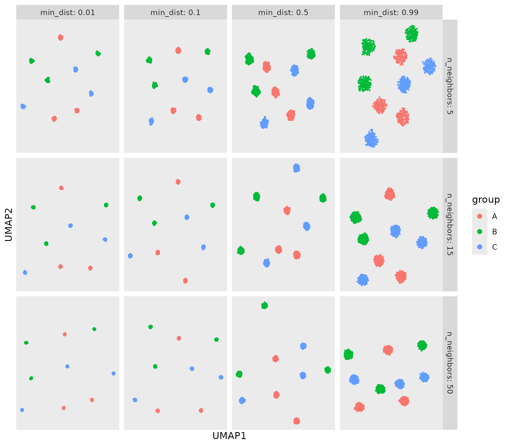
Within a plot, you would write each of these as a single layer, e.g.
Distance metrics
metric defines distances in the input space. Cosine and
correlation distances ignore the magnitude of the feature vectors, which
is useful for text embeddings, counts and other data where only the
direction matters.
metrics <- c("euclidean", "manhattan", "cosine", "correlation")
by_metric <- do.call(rbind, lapply(metrics, function(m) {
  emb <- umap_embed(df, starts_with("X"), metric = m, seed = 1)
  cbind(emb, df["group"], metric = m)
}))
ggplot(by_metric, aes(UMAP1, UMAP2, colour = group)) +
  geom_point(size = 0.3) +
  facet_wrap(vars(metric), nrow = 1, scales = "free") +
  theme_umap()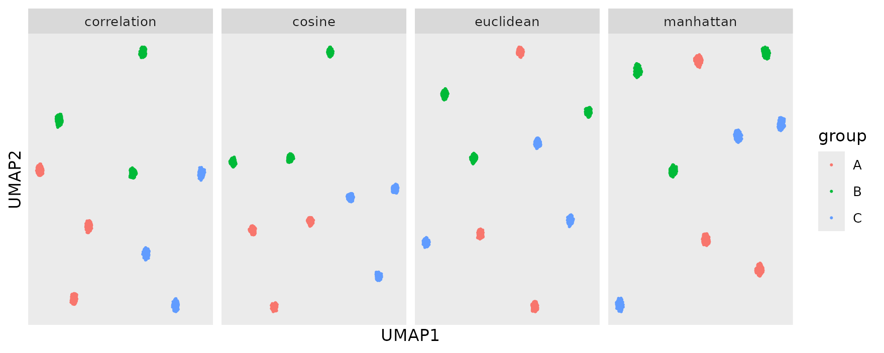
Flavour and initialisation
flavour = "0.5" (the default) reproduces the classic
umap-learn pipeline: a spectral initialisation followed by stochastic
gradient descent. flavour = "0.6" uses umap-learn 0.6’s
recursive initialisation and the Adam optimiser; it is faster and
deterministic for a fixed number of threads. init overrides
the initialisation of either flavour.
combos <- expand.grid(flavour = c("0.5", "0.6"), init = c("auto", "pca", "random"), stringsAsFactors = FALSE)
by_flavour <- do.call(rbind, Map(function(f, i) {
  emb <- umap_embed(df, starts_with("X"), flavour = f, init = i, seed = 1)
  cbind(emb, df["group"], flavour = f, init = i)
}, combos$flavour, combos$init))
ggplot(by_flavour, aes(UMAP1, UMAP2, colour = group)) +
  geom_point(size = 0.3) +
  facet_grid(vars(flavour), vars(init), scales = "free", labeller = label_both) +
  theme_umap()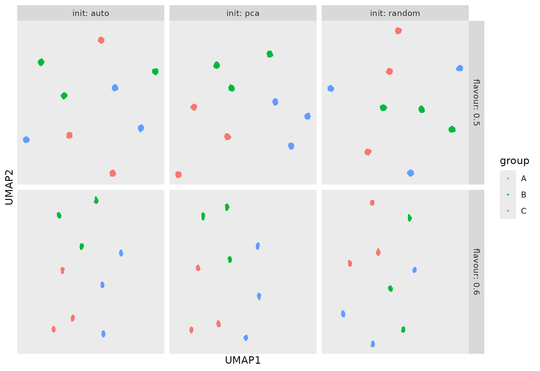
Scaling
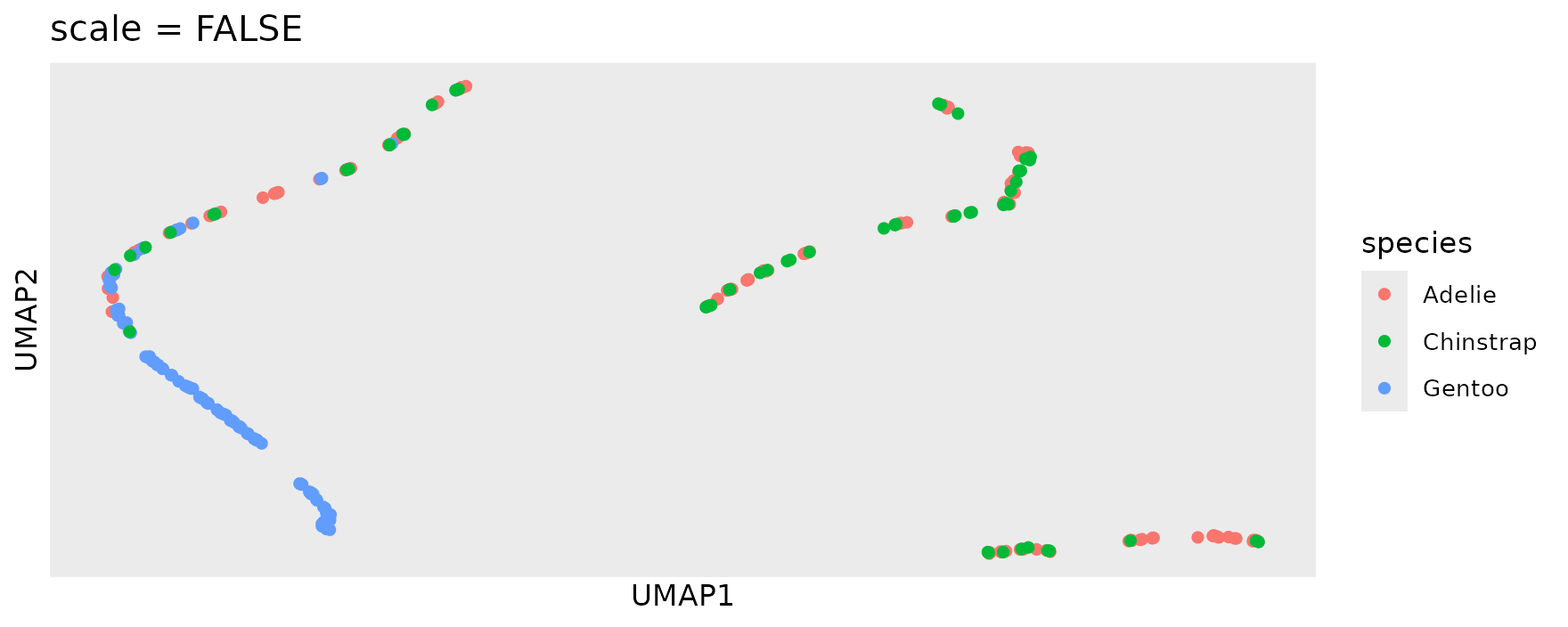
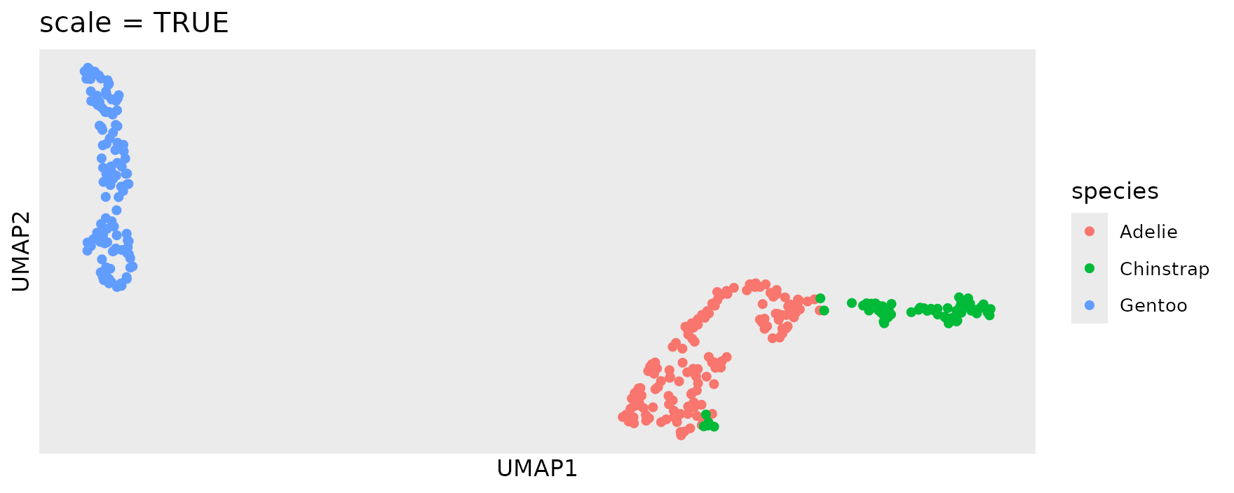
UMAP uses the features as they are. When they are measured in
different units, the feature with the largest range dominates the
distances. scale = TRUE standardises every feature
first.
penguins <- palmerpenguins::penguins
p <- ggplot(penguins, aes(colour = species)) + theme_umap()
patch <- list(
  p + geom_umap(features = bill_length_mm:body_mass_g, na.rm = TRUE) + ggtitle("scale = FALSE"),
  p + geom_umap(features = bill_length_mm:body_mass_g, scale = TRUE, na.rm = TRUE) + ggtitle("scale = TRUE")
)
has_patchwork <- requireNamespace("patchwork", quietly = TRUE)
if (has_patchwork) {
  patchwork::wrap_plots(patch, guides = "collect")
} else {
  for (pl in patch) print(pl)
}
Advanced settings
umap_control() holds the remaining parameters of the
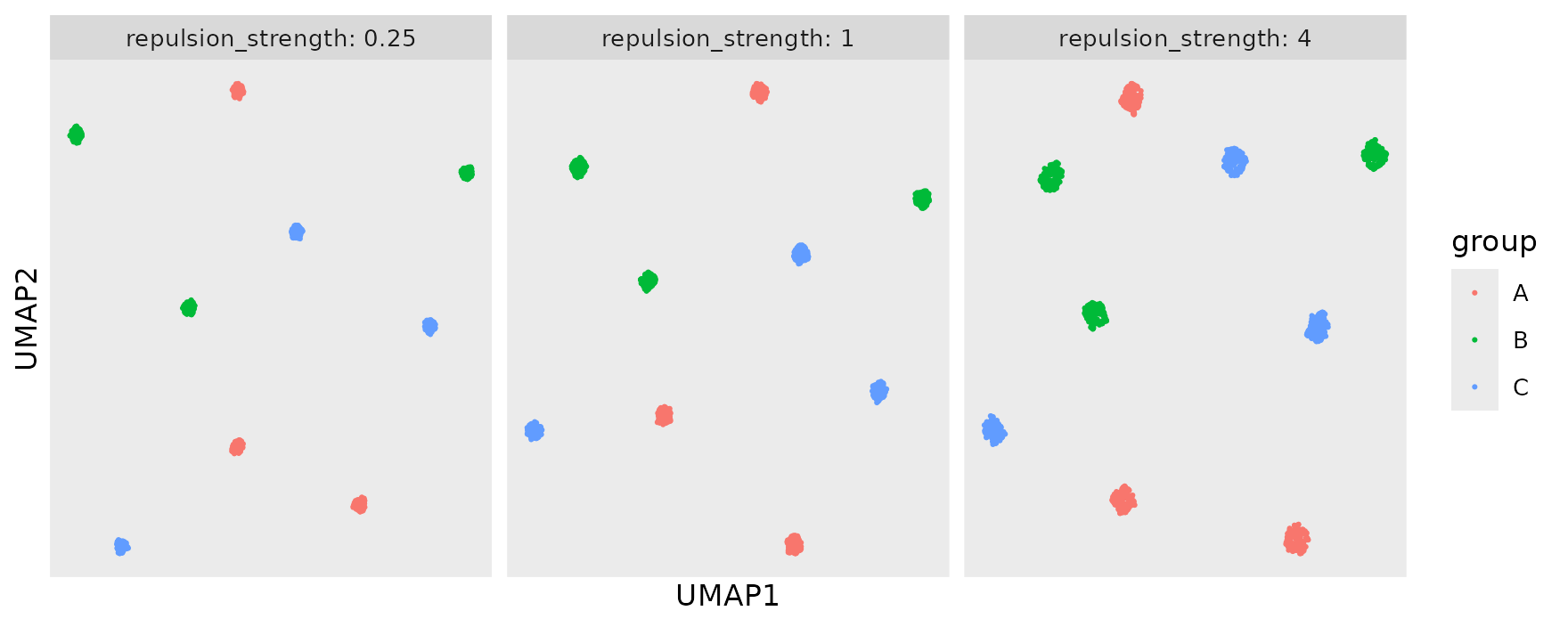
algorithm. The most useful are repulsion_strength (how
strongly unrelated points repel each other) and
negative_sample_rate (how many repulsive samples are drawn
per attractive one).
strengths <- c(0.25, 1, 4)
by_strength <- do.call(rbind, lapply(strengths, function(s) {
  emb <- umap_embed(df, starts_with("X"), seed = 1, control = umap_control(repulsion_strength = s))
  cbind(emb, df["group"], repulsion_strength = s)
}))
ggplot(by_strength, aes(UMAP1, UMAP2, colour = group)) +
  geom_point(size = 0.3) +
  facet_wrap(vars(repulsion_strength), labeller = label_both, scales = "free") +
  theme_umap()