UMAP (Uniform Manifold Approximation and Projection) embeds high-dimensional data in two dimensions, preserving which observations are close to each other. ggumap computes the embedding inside a ggplot2 layer, so there is no separate step and no data wrangling between computation and plot.
A first plot
geom_umap() uses all numeric columns as features and
draws points. Aesthetics like colour work as usual; they
are carried along, but do not influence the embedding.
penguins <- palmerpenguins::penguins

ggplot(penguins, aes(colour = species)) +
  geom_umap(na.rm = TRUE)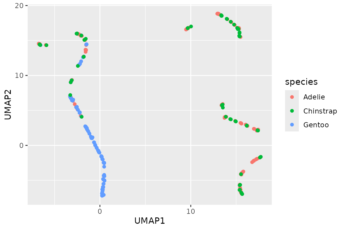
The numeric columns of penguins are measured in
different units (body mass in grams dominates the distances), so
standardise them with scale = TRUE.
theme_umap() removes axis text and ticks, since UMAP
coordinates have no meaning of their own.
ggplot(penguins, aes(colour = species)) +
  geom_umap(scale = TRUE, na.rm = TRUE) +
  theme_umap()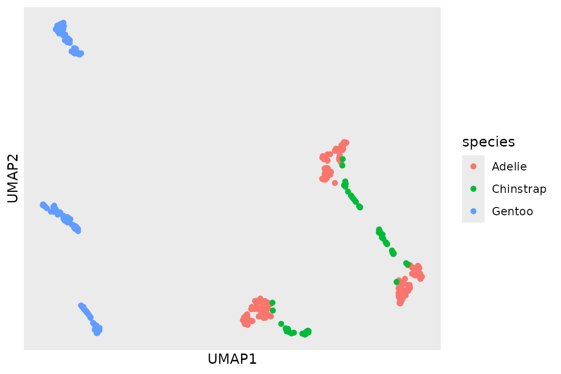
Selecting features
features takes the same syntax as
dplyr::select(). Here year is left out:
ggplot(penguins, aes(colour = species, shape = sex)) +
  geom_umap(features = bill_length_mm:body_mass_g, scale = TRUE, na.rm = TRUE) +
  theme_umap()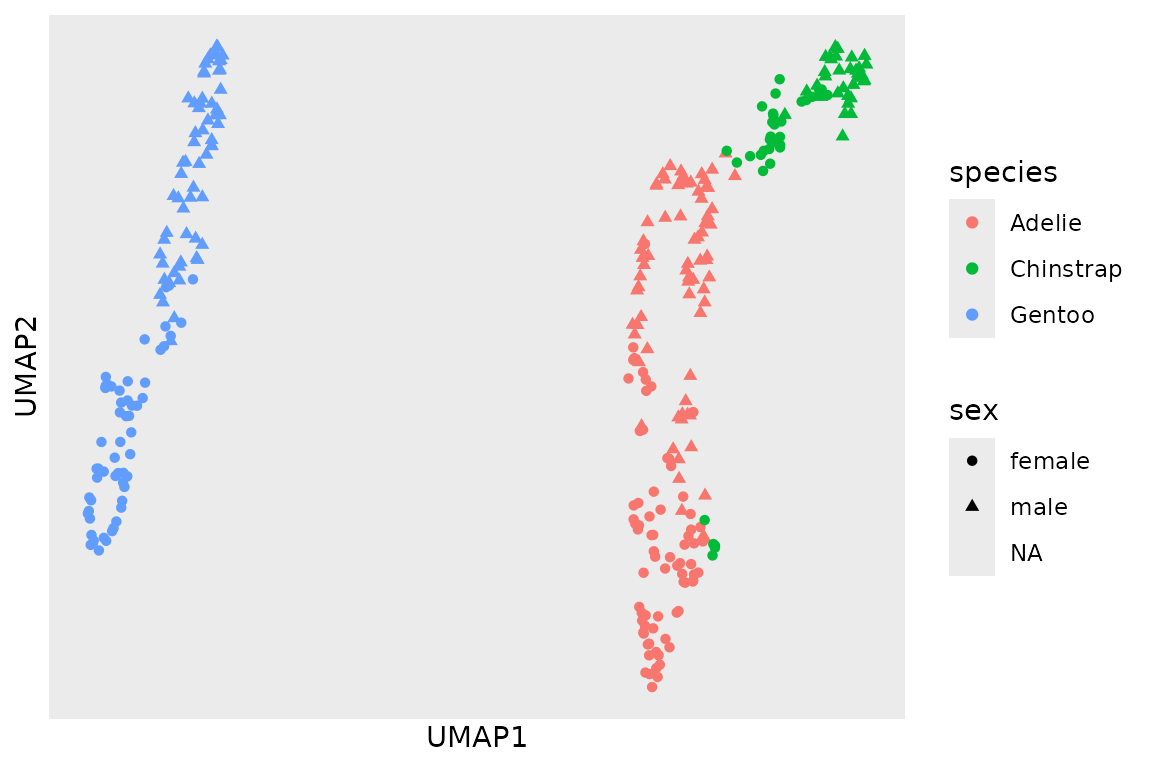
Any geom, several layers
stat_umap() can render the embedding with any geom.
Layers with the same data and settings share one embedding: it is
computed once and cached.
cars <- transform(mtcars, model = rownames(mtcars))

ggplot(cars, aes(label = model, colour = factor(cyl))) +
  geom_umap(scale = TRUE, n_neighbors = 5) +
  stat_umap(
    geom = "text", scale = TRUE, n_neighbors = 5,
    size = 2.5, vjust = -0.8, show.legend = FALSE,
    check_overlap = TRUE
  ) +
  scale_x_continuous(expand = expansion(mult = 0.15)) +
  labs(colour = "cylinders") +
  theme_umap()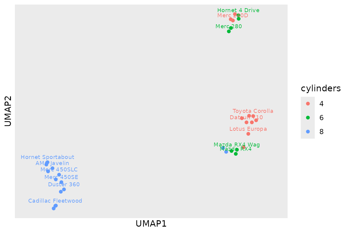
ggplot(penguins) +
  stat_umap(
    geom = "density_2d_filled", features = bill_length_mm:body_mass_g,
    scale = TRUE, na.rm = TRUE, contour_var = "ndensity"
  ) +
  theme_umap()
#> Warning in umap_layer(mapping = mapping, data = data, geom = geom, position =
#> position, : Ignoring unknown parameters: `contour_var`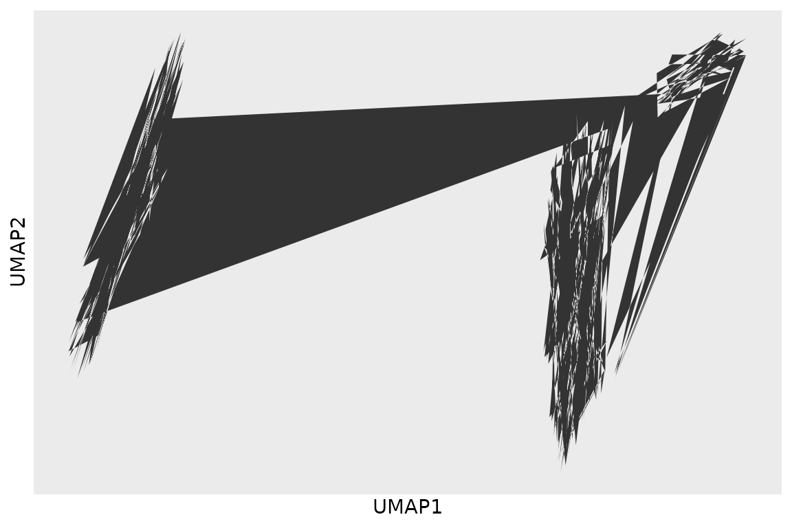
Computed variables
Besides the coordinates UMAP1 and UMAP2,
the stat computes knn_dist, the mean distance of each
observation to its nearest neighbours in the input space. Large values
point at outliers.
ggplot(penguins) +
  geom_umap(
    aes(colour = after_stat(knn_dist)),
    features = bill_length_mm:body_mass_g, scale = TRUE, na.rm = TRUE
  ) +
  scale_colour_viridis_c() +
  theme_umap()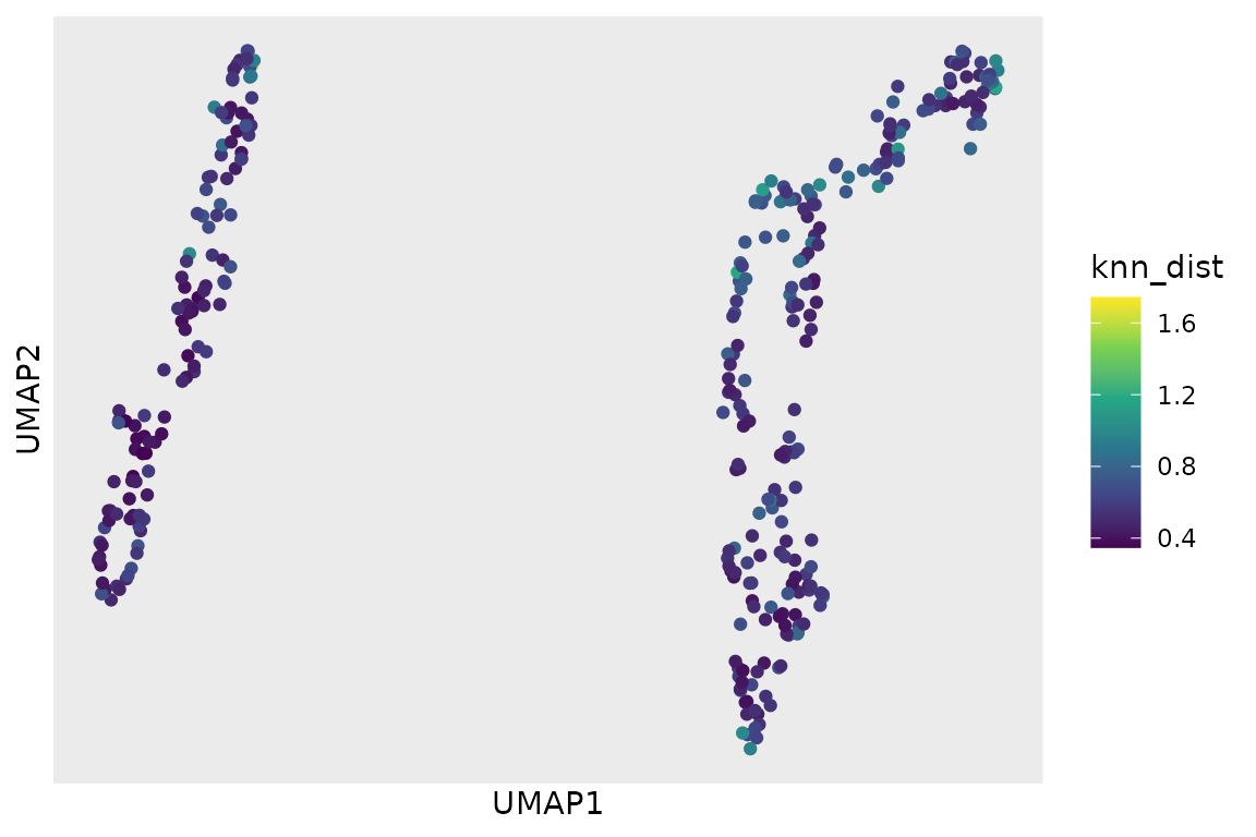
Facets
By default one embedding is computed for the whole layer, and each
facet shows a subset of it. With scope = "panel", every
panel gets its own embedding.
ggplot(penguins, aes(colour = sex)) +
  geom_umap(features = bill_length_mm:body_mass_g, scale = TRUE, na.rm = TRUE) +
  facet_wrap(vars(species)) +
  theme_umap()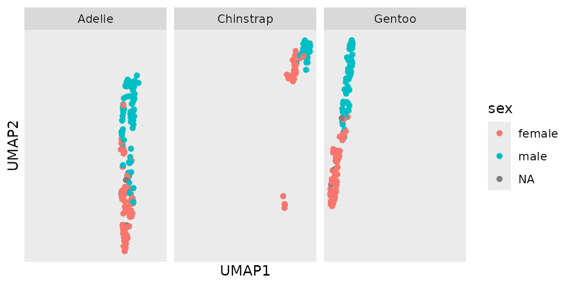
Tuning UMAP
The most important parameters are
-
n_neighbors: the size of the neighbourhood. Small values emphasise local structure, large values global structure. -
min_dist: how tightly points may be packed together. -
metric: the distance in input space, e.g."cosine"or"manhattan".
ggplot(penguins, aes(colour = species)) +
  geom_umap(
    features = bill_length_mm:body_mass_g, scale = TRUE, na.rm = TRUE,
    n_neighbors = 50, min_dist = 0.8
  ) +
  theme_umap()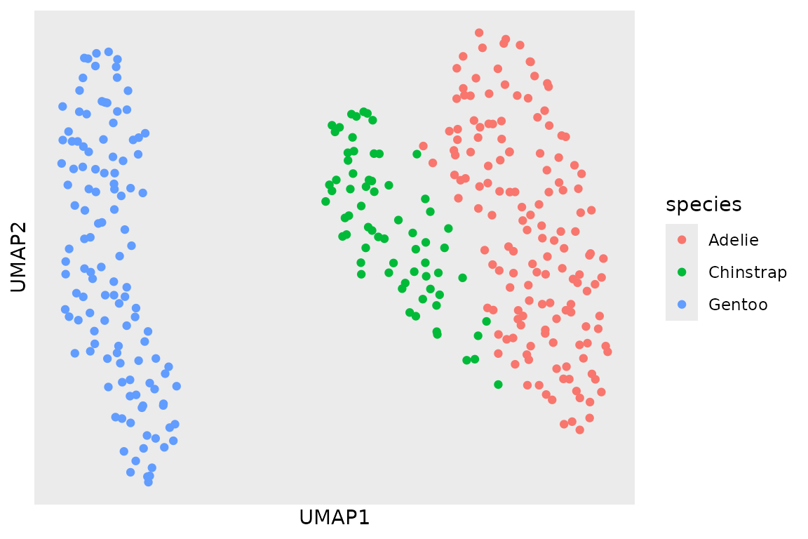
Rarely needed parameters live in umap_control().
Reproducibility
The stat derives its random seed from the data, so a plot looks the
same every time it is drawn. Pass seed to choose another
layout:
ggplot(penguins, aes(colour = species)) +
  geom_umap(
    features = bill_length_mm:body_mass_g, scale = TRUE, na.rm = TRUE,
    seed = 2
  ) +
  theme_umap()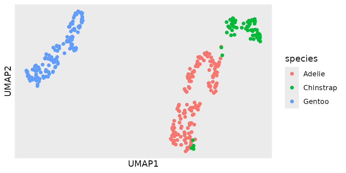
UMAP runs in parallel on umap_threads() threads (half of
your cores by default; set the option ggumap.n_threads to
change this). With the default flavour = "0.5",
multi-threaded results are not bit-for-bit reproducible across sessions;
use n_threads = 1, or flavour = "0.6" which is
deterministic for a fixed number of threads.
Outside of plots
umap_embed() returns the embedding as a data frame, for
example to use it in further analyses:
emb <- umap_embed(penguins, bill_length_mm:body_mass_g, scale = TRUE, seed = 1)
#> Warning: 2 rows with missing feature values were not embedded.
head(emb)
#>       UMAP1    UMAP2  knn_dist
#> 1 10.272740 4.840488 0.4845237
#> 2  9.229644 5.399489 0.4829426
#> 3  8.558975 5.213395 0.5710326
#> 4        NA       NA        NA
#> 5 10.881407 4.062928 0.5631385
#> 6 12.290913 4.057639 0.6878517